Philipp
Backtesting Trading Strategies Using Python
Over the past several decades, the use of machines for exploring and developing new investing and trading strategies in financial markets has exploded. Instead of relying on humans, we can instead come up with some sort of strategy (or even have a machine find one) and tell the computer exactly how and when to execute it.
However, we need to make sure our strategy is feasible to begin with. The most straightforward way is to see how our strategy would have performed historically based on prior market data, also known as a backtest. Think about it outside the context of finance - before buying a product online, you’d generally look at the reviews, ratings, see other people’s experiences with it before you go ahead and buy it yourself - why not do the same with financial assets?
In addition, through a backtest we can get a much clearer picture of exactly how much money we’d have made, at what levels of volatility, daily/monthly/annual averages, our actual annualized growth rate, etc.
Various tools and services exist for backtesting and the data necessary for it, however here I’m going to go over implementation of backtests of several strategies using the bt Python backtesting library with historical data from Yahoo Finance.
Strategies - A Primer
Before we backtest a strategy, we actually need to have one. And to have a strategy, we need to define our goals. Obviously our goal is to make money, but we need to be more specific about this.
Let’s say we do come up with something, and it’s profitable, yielding 3% or so a year. Why would we invest in that strategy instead of just putting our money into a fund that tracks the S&P 500, which has yielded ~9% a year annualized since the 1950s, with significantly less time and effort?
Not only do we need to be profitable, but we need to be profitable enough that it’s worth the risk and opportunity cost of just buying SPY, VFIAX, FZROX etc., or some 60/40 stock/bond blend. In other words, we’d like to beat the benchmark.
We also need to think about how we’re achieving our goals. Are we being smarter about asset allocation? Is there some signal or some piece of information that can indicate a large sell off? Or a large rally? Are we exploiting some consistent mispricing or a particular arbitrage scenario? Are we scanning the market for all equities and trading the ones that fit some sort of criteria that would fit our strategy, or are we looking at trading only a couple of instruments in a specific way?
Even figuring something out that matches S&P500 returns annually, but at lower risk (lower volatility, smaller drawdowns) would be a big win. Since every time we buy equities we’re putting money at risk, generating similar returns with a much more attractive risk profile is a large positive. Conversely, generating much better returns might force us to take on more risk. Remember the classic risk reward curve.
In addition, we need to be aware of any biases we could have when designing a new strategy. Of course we could backtest something which only buys Domino’s Pizza (DPZ), say we’re a genius, and go forward with that strategy. We should ensure that our idea works and makes decisions based only on data it would have at that time (eliminate look-ahead bias). It’s also important to remember that past performance is not indicative of future returns. Everything could change, and individual strategies can stop becoming profitable at any time.
That being said, for the purposes of this post, I’m going to propose several simple strategies that we can use just to get a feel for the tooling and workflow of backtesting. However, the questions and points I highlighted are important to think about as they define what kind of data we’re going to need and how we’re going to design our tests.
Proposed Strategies
I’m going to go over the following, which should hopefully give you enough examples to come up with your own:
- Benchmark:
- Pure long, buy and hold SPY
- Strategy 1:
- Maintain a 70/30 SPY/VIRT portfolio and rebalance daily
- Strategy 2:
- Equal weight portfolio of SPY, QQQ, TLT, and GLD, rebalanced monthly.
- Strategy 3:
- 100% SPY, but sell half when SPY goes up more than 2% in one day, and rebuy half only when SPY goes down more than 2% in one day.
- Strategy 4:
- Monitor VIX futures and index prices daily, and either go long or short UVXY based on whether or not VIX is in contango, e.g. short UVXY by default, and long UVXY if the front future (greater than 30 days) is cheaper than the current index “price” by more than 10%. Then, balance this strategy allocation equally with just long SPY daily.
Getting Data
Before we go ahead implementing our strategies, we need to get historical data for the instruments we’re interested in. Looking at what we’ve proposed above, we’ll need daily data for SPY, VIRT, QQQ, TLT, GLD, UVXY. For the last strategy, we’ll also need the VIX index and every VIX future we can get.
As I mentioned, I’ll show you how to do this using Yahoo Finance data. Yahoo Finance data isn’t the highest quality, and we’re limited to daily data only, but it is free and easily accessible. In a follow-up post, I’ll show you how to use the Interactive Brokers (IBKR) API to get historical and live data. IBKR provides data of various types of frequencies, from tick-by-tick to yearly, for a variety of instruments.
Yahoo Finance Data
There’s several ways to do this. The most direct way is probably scraping the site itself, but that can be a lot of work. Fortunately, there are libraries that exist for this purpose already, such as yfinance.
We’ll also be using pandas (for dataframe manipulation), bt (for backtesting), and matplotlib (for plotting) later, so if you don’t have them, you should install them now by running pip install pandas bt yfinance matplotlib in your terminal. I’m going to keep them imported in all the examples for consistency.
Following the documentation, we could do something like this:
import bt
import pandas as pd
import yfinance as yf
import matplotlib.pyplot as plt

spy = yf.Ticker('SPY')

spy_data = spy.history(period='max')

print(spy_data)
and we can see that we get the historical prices of the SPY ETF since 1993-01-29.
                  Open        High         Low       Close     Volume  Dividends  Stock Splits
Date
1993-01-29   25.645566   25.645566   25.517976   25.627338    1003200        0.0             0
1993-02-01   25.645566   25.809610   25.645566   25.809610     480500        0.0             0
1993-02-02   25.791405   25.882540   25.736723   25.864313     201300        0.0             0
1993-02-03   25.900752   26.155932   25.882525   26.137705     529400        0.0             0
1993-02-04   26.228843   26.301752   25.937209   26.247070     531500        0.0             0
...                ...         ...         ...         ...        ...        ...           ...
2022-01-10  462.700012  465.739990  456.600006  465.510010  119362000        0.0             0
2022-01-11  465.230011  469.850006  462.049988  469.750000   74303100        0.0             0
2022-01-12  471.589996  473.200012  468.940002  471.019989   67605400        0.0             0
2022-01-13  472.190002  472.880005  463.440002  464.529999   91173100        0.0             0
2022-01-14  461.190002  465.089996  459.899994  464.720001   95849600        0.0             0

[7295 rows x 7 columns]
We can repeat this for every ticker, and in fact we can just functionalize this and collect all of them at once.
import bt
import pandas as pd
import yfinance as yf
import matplotlib.pyplot as plt

# The tickers we're interested in
tickers = [
    'SPY',
    'VIRT',
    'QQQ',
    'TLT',
    'GLD',
    'UVXY',
    '^VIX'
]

# Get maximum historical data for a single ticker
def get_yf_hist(ticker):
    data = yf.Ticker(ticker).history(period='max')
    return data

# For each ticker, get the historical data and add it to a list
def get_data_for_tickers(tickers):
    data = []
    for ticker in tickers:
        data.append(get_yf_hist(ticker))
    return data

# Get our list of data per ticker
data = get_data_for_tickers(tickers)
and now we have a list of Pandas DataFrames, each with maximum historical data for each asset.
An important note here - how are we going to be using this data in our strategies? Are we going to be relying on just closing prices every day? Do we need the open, the high, the low? Are we interested in volume?
For simplicity, we’re going to run everything based on closing prices only. This is just an assumption, however, as the closing prices every day indicate the last trade price before the market closed - it’s not guaranteed that we would be able to execute our trades at that price for whatever volume we’re looking for.
For something as liquid as SPY or QQQ, it might be possible, but for less liquid stocks (e.g. VIRT), we might not get a fill at that price for the day. This is especially more relevant if you’re testing against options data, where even a relatively liquid stock might have a fairly illiquid options market. Just something to keep in mind.
So, to filter closing prices only, we’d want to only keep the column in our dataframes that corresponds to the closing price. We can just filter the column by changing our get_yf_hist function to only keep ['Close'].
So this
def get_yf_hist(ticker):
    data = yf.Ticker(ticker).history(period='max')
    return data
becomes this
def get_yf_hist(ticker):
    data = yf.Ticker(ticker).history(period='max')['Close']
    return data
And since we’re only keeping the one column, we probably want to rename the column so we can differentiate them from the other datasets, as if you’ll notice they weren’t named.
When we select the column by selecting only ['Close'], we get a Pandas Series, not a separate dataframe, so we can just rename the series.
Our above segment now becomes this
def get_yf_hist(ticker):
    data = yf.Ticker(ticker).history(period='max')['Close']
    data.rename(ticker, inplace=True)
    return data
I use the inplace=True argument here, so we don’t have to reassign the series.
Finally, we should probably gather all of these separate series and concatenate them into one dataframe for simplicity.
However, since every instrument has a different starting date, e.g. VIRT’s first day of trading was 2015-04-16 while TLT’s was 2002-07-30, we can’t just add these records starting at the same time.
Notice that every data series we get back has an Index, which we can use to keep all of our records in order. We’ll be able to then use the maximum amount of data for each separate strategy, while keeping everything associated with its correct date.
Thus, we can use the built in pandas function pd.concat to stitch our series together. We want to make sure we concatenate along the columns, not the index, so we use axis=1 as an argument here.
We can do this by changing the function get_data_for_tickers from this
def get_data_for_tickers(tickers):
    data = []
    for ticker in tickers:
        data.append(get_yf_hist(ticker))
    return data
to this
def get_data_for_tickers(tickers):
    data = []
    for ticker in tickers:
        data.append(get_yf_hist(ticker))
    df = pd.concat(data, axis=1)
    return df
So far, our data collection should look like this:
import bt
import pandas as pd
import yfinance as yf
import matplotlib.pyplot as plt

# The tickers we're interested in
tickers = [
    'SPY',
    'VIRT',
    'QQQ',
    'TLT',
    'GLD',
    'UVXY',
    '^VIX'
]

# Get maximum historical data for a single ticker
def get_yf_hist(ticker):
    data = yf.Ticker(ticker).history(period='max')['Close']
    data.rename(ticker, inplace=True)
    return data

# For each ticker, get the historical data and add it to a list
def get_data_for_tickers(tickers):
    data = []
    for ticker in tickers:
        data.append(get_yf_hist(ticker))
    df = pd.concat(data, axis=1)
    return df

data = get_data_for_tickers(tickers)
print(data)
Now, if we run our whole process, we’ll see that we get a properly stitched together dataframe, with each ticker’s closing price in its own column, all aligned by date. Perfect.
                   SPY       VIRT         QQQ         TLT         GLD   UVXY       ^VIX
Date
1990-01-02         NaN        NaN         NaN         NaN         NaN    NaN  17.240000
1990-01-03         NaN        NaN         NaN         NaN         NaN    NaN  18.190001
1990-01-04         NaN        NaN         NaN         NaN         NaN    NaN  19.219999
1990-01-05         NaN        NaN         NaN         NaN         NaN    NaN  20.110001
1990-01-08         NaN        NaN         NaN         NaN         NaN    NaN  20.260000
...                ...        ...         ...         ...         ...    ...        ...
2022-01-10  465.510010  30.330000  380.109985  142.610001  168.259995  12.35  19.400000
2022-01-11  469.750000  30.959999  385.820007  143.559998  170.289993  11.67  18.410000
2022-01-12  471.019989  30.809999  387.350006  143.009995  170.740005  11.51  17.620001
2022-01-13  464.529999  29.549999  377.660004  144.279999  170.160004  12.55  20.309999
2022-01-14  464.720001  29.070000  380.010010  142.100006  169.669998  12.28  19.190001

[8074 rows x 7 columns]
For the purposes of backtesting strategies that run at most daily, we now have all the data we need. We can move on to actually integrating this into a backtest.
Backtesting
As mentioned previously, we’ll be using the bt backtesting library. There a variety of them out there, including backtrader, zipline, pandas-ta, etc. I found a small list (not maintained by me) that showcases libraries that fit this purpose.
It’s also possible to write your own, and perhaps its best to do so, but it’s a significant time investment; until we really need to, we should probably avoid reinventing the wheel and stick to using an existing library.
Let’s go ahead and get started with bt. From the documentation, we can also see that bt actually has its own method of getting historical data from Yahoo Finance for assets!
(From the main documentation page)
import bt

data = bt.get('SPY,AGG', start='2010-01-01')
print(data)
                   spy         agg
Date
2010-01-04   89.889206   75.541451
2010-01-05   90.127174   75.885139
2010-01-06   90.190628   75.841270
2010-01-07   90.571365   75.753487
2010-01-08   90.872734   75.797394
...                ...         ...
2022-01-10  465.510010  112.389999
2022-01-11  469.750000  112.599998
2022-01-12  471.019989  112.599998
2022-01-13  464.529999  112.800003
2022-01-14  464.720001  112.169998

[3031 rows x 2 columns]
Which probably brings you to ask - why did we spend time covering downloading data from yfinance previously?
While closing prices are fine for the purposes of this post, you might want to integrate other sources of data. Perhaps you’re interested in something that looks at not just the close, but the open and the high too. Or you want to integrate additional data related to a stock that’s not just prices, such as volume or some sort of social sentiment attached to the stock. Or you want data at higher frequency, or you already have higher quality data from other sources (such as IBKR).
Using the methods I described above, we could attach those extra fields, and extend the above logic to use that data in our backtests. Let’s stick with our yfinance method for now, but feel free to experiment with the bt data.
Now, let’s actually use bt to define and test our strategies.
Benchmark - Buy And Hold SPY
Let’s start with our benchmark - simply buying and holding SPY since inception.
In bt, it would look something like this:
# The name of our strategy
name = 'long_spy'

# Defining the actual strategy
benchmark_strat = bt.Strategy(
    name,
    [
        bt.algos.RunOnce(),
        bt.algos.SelectAll(),
        bt.algos.WeighEqually(),
        bt.algos.Rebalance()
    ]
)

# Make sure we're only running on the SPY data by selecting it out,
# and dropping the rows for which we have no data
spy_data = data[['SPY']]
spy_data.dropna(inplace=True)

# Generate the backtest using the defined strategy and data and run it
benchmark_test = bt.Backtest(benchmark_strat, spy_data)
res = bt.run(benchmark_test)

# Print the summary and plot our equity progression
res.plot()
res.display()
plt.show()
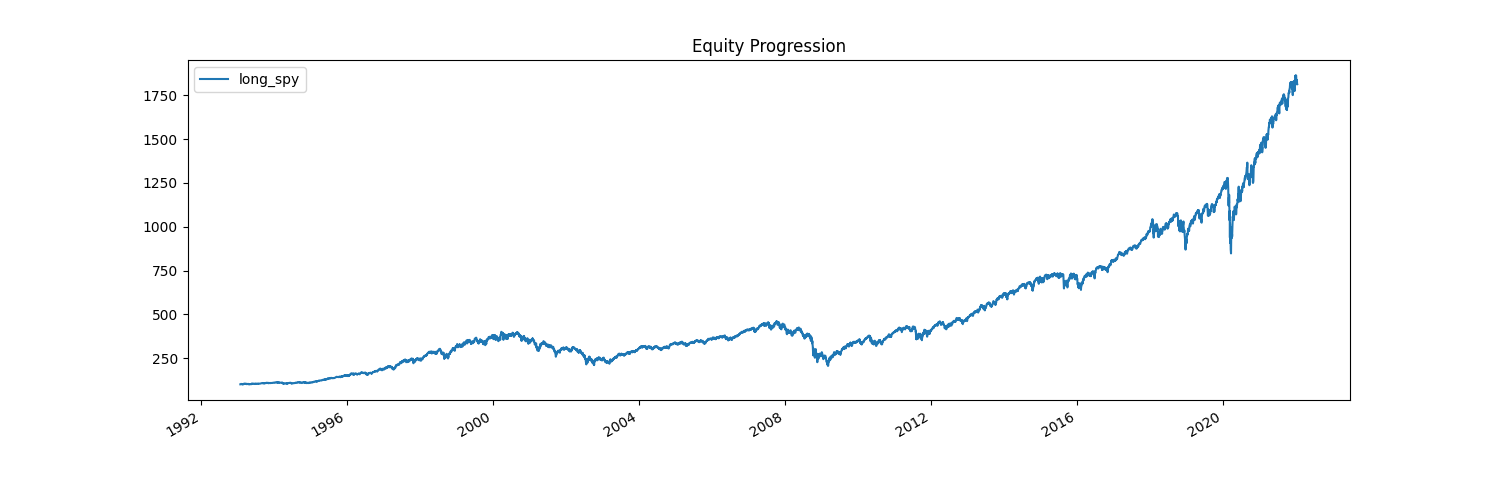
Pretty cool! We can see how our strategy’s value has progressed over time (which is exactly the historical SPY chart), and we get a table full of summary statistics.
Stat                 long_spy
-------------------  ----------
Start                1993-01-28
End                  2022-01-14
Risk-free rate       0.00%

Total Return         1713.34%
Daily Sharpe         0.63
Daily Sortino        0.99
CAGR                 10.52%
Max Drawdown         -55.19%
Calmar Ratio         0.19

MTD                  -2.16%
3m                   5.39%
6m                   7.25%
YTD                  -2.16%
1Y                   24.43%
3Y (ann.)            23.83%
5Y (ann.)            17.58%
10Y (ann.)           15.85%
Since Incep. (ann.)  10.52%

Daily Sharpe         0.63
Daily Sortino        0.99
Daily Mean (ann.)    11.76%
Daily Vol (ann.)     18.71%
Daily Skew           -0.06
Daily Kurt           12.15
Best Day             14.52%
Worst Day            -10.94%

Monthly Sharpe       0.76
Monthly Sortino      1.29
Monthly Mean (ann.)  11.10%
Monthly Vol (ann.)   14.57%
Monthly Skew         -0.62
Monthly Kurt         1.27
Best Month           12.70%
Worst Month          -16.52%

Yearly Sharpe        0.66
Yearly Sortino       1.45
Yearly Mean          11.72%
Yearly Vol           17.70%
Yearly Skew          -0.83
Yearly Kurt          0.61
Best Year            38.05%
Worst Year           -36.79%

Avg. Drawdown        -1.87%
Avg. Drawdown Days   25.49
Avg. Up Month        3.29%
Avg. Down Month      -3.51%
Win Year %           79.31%
Win 12m %            82.25%
Now, what’s actually going on when we define strategy_1?
benchmark_strat = bt.Strategy(
    name,
    [
        bt.algos.RunOnce(),
        bt.algos.SelectAll(),
        bt.algos.WeighEqually(),
        bt.algos.Rebalance()
    ]
)
First, every strategy needs a name. This is due to the fact that we can actually reuse this strategy as a component in a different strategy, which we’ll cover in a little bit.
Then, we have a list of different bt algos. I’ll go over the ones in use here and in further strategies, but I can’t cover them all. If you’re curious, check out the documentation to see everything available.
Starting with bt.algos.RunOnce(), this just tells bt that we only need to run the algo once. This is useful in situations such as our current one, where we are only buying and holding.
bt.algos.SelectAll() just means that we want to test all securities in the given data. We already filtered only for SPY, but we still need to tell bt to include all securities (even if it’s just one). If, for example, we passed in SPY and TLT, it would include both of them in the strategy.
bt.algos.WeighEqually() means that, of all the securities we selected, we need to give each of them the same allocation in our strategy. Again, since we only have one instrument, it’s going to allocate 100%. Alternatively, we could also do something like:
bt.algos.WeighSpecified(SPY=1.0)
which would set SPY to have a 100% allocation. Indeed, if you run this, you’ll see the exact same results.
Finally, we have bt.algos.Rebalance(). This just means that we want, for every period we see in the data (every day), to rebalance the portfolio such that each instrument has an allocation matching the weights we specified.
Again, since we only have one instrument, and we only buy things once, this isn’t as relevant but still necessary. Why? Because at the start of day 1, we have 100% cash and 0% SPY. We need to actually tell our strategy how to allocate our capital, e.g. rebalance into 0% cash and 100% SPY.
Having done the benchmark, we can now move on to our first real strategy.
Strategy 1 - Maintain a 70/30 SPY/VIRT portfolio and rebalance daily
Using the benchmark example, we can actually reuse a lot of the logic we have there. We need to make sure we’re selecting both SPY and VIRT from our data, we need to set the target weights appropriately, and we need it to run daily.
name = 'spy_virt_7030'

strategy_1 = bt.Strategy(
    name,
    [
        bt.algos.RunDaily(),
        bt.algos.SelectAll(),
        bt.algos.WeighSpecified(SPY=0.7, VIRT=0.3),
        bt.algos.Rebalance()
    ]
)

spy_virt_data = data[['SPY', 'VIRT']]
spy_virt_data.dropna(inplace=True)

backtest_1 = bt.Backtest(strategy_1, spy_virt_data)
res = bt.run(backtest_1)

res.plot()
res.display()
plt.show()
A lot of this should look familiar. We’re running daily now, as specified, and we’re selecting all of the instruments. We’re weighing them with a specific target weight (as mentioned earlier) and rebalancing every period (daily).
However, how do we know how well we’re doing?
We can just include our previous benchmark strategy we created and run it alongside our newly defined one:
res = bt.run(backtest_1, benchmark_test)

res.plot()
res.display()
plt.show()
Stat                 spy_virt_7030    long_spy
-------------------  ---------------  ----------
Start                2015-04-15       2015-04-15
End                  2022-01-14       2022-01-14
Risk-free rate       0.00%            0.00%

Total Return         152.36%          150.45%
Daily Sharpe         0.89             0.85
Daily Sortino        1.45             1.28
CAGR                 14.70%           14.57%
Max Drawdown         -21.75%          -33.72%
Calmar Ratio         0.68             0.43

MTD                  -1.23%           -2.16%
3m                   8.87%            5.39%
6m                   9.61%            7.25%
YTD                  -1.23%           -2.16%
1Y                   25.10%           24.43%
3Y (ann.)            21.07%           23.83%
5Y (ann.)            19.85%           17.58%
10Y (ann.)           -                -
Since Incep. (ann.)  14.70%           14.57%

Daily Sharpe         0.89             0.85
Daily Sortino        1.45             1.28
Daily Mean (ann.)    15.16%           15.19%
Daily Vol (ann.)     17.05%           17.81%
Daily Skew           -0.23            -0.73
Daily Kurt           10.24            17.32
Best Day             7.03%            9.06%
Worst Day            -8.56%           -10.94%

Monthly Sharpe       1.06             1.02
Monthly Sortino      2.52             1.82
Monthly Mean (ann.)  15.01%           14.86%
Monthly Vol (ann.)   14.18%           14.53%
Monthly Skew         0.45             -0.42
Monthly Kurt         0.27             1.47
Best Month           12.98%           12.70%
Worst Month          -5.94%           -12.49%

Yearly Sharpe        1.07             1.07
Yearly Sortino       31.58            8.44
Yearly Mean          14.68%           15.04%
Yearly Vol           13.77%           14.11%
Yearly Skew          0.24             -0.46
Yearly Kurt          -1.60            -1.38
Best Year            34.44%           31.22%
Worst Year           -1.23%           -4.57%

Avg. Drawdown        -2.44%           -1.51%
Avg. Drawdown Days   26.81            14.38
Avg. Up Month        4.01%            3.14%
Avg. Down Month      -2.57%           -3.85%
Win Year %           85.71%           71.43%
Win 12m %            84.51%           95.77%
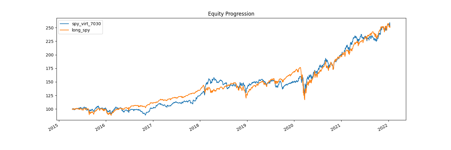
Right away, we can see how our strategy compares to our benchmark. Visually, our equity progression isn’t much different from our benchmark. In fact, it seems like we’re underperforming a fair amount of time. However, we don’t lose as much when SPY goes down.
This is where our summary statistics are incredibly helpful. We can see that overall, we’ve actually beaten the benchmark, but not by much. The CAGR is higher by not even half a percent. The interesting thing here is that our drawdown is significantly lower than SPY! Indeed, our daily, monthly, and annual volatility is measurably lower. Our worst year yielded nothing, while SPY suffered nearly 5%. However, we do drawdown for longer periods of time, nearly double that of SPY.
An important note: if you noticed, this test as compared to the benchmark only runs for data since 2015 - this is because VIRT has only been public since then, and we need the prices of both assets to allocate to them. One thing to consider is that our test could be biased - the S&P for that time has been in an extraordinary bull market, and who knows if this strategy would work under different market conditions?
Also, we have to consider the practical implementation of this - would we really beat SPY? If we have to rebalance daily, we might also have to consider the cost of executing these trades (since we have to pay commission). What if we wanted to maybe rebalance monthly? This brings us to the next strategy.
Strategy 2 - Equal weight portfolio of SPY, QQQ, TLT, and GLD, rebalanced monthly
name = 'eq_wt_monthly'

strategy_2 = bt.Strategy(
    name,
    [
        bt.algos.RunMonthly(),
        bt.algos.SelectAll(),
        bt.algos.WeighEqually(),
        bt.algos.Rebalance()
    ]
)

eq_wt_data = data[['SPY', 'QQQ', 'TLT', 'GLD']]
eq_wt_data.dropna(inplace=True)

backtest_2 = bt.Backtest(strategy_2, eq_wt_data)
res = bt.run(backtest_2, benchmark_test)

res.plot()
res.display()
plt.show()
Again, most of this should look familiar by now. We set a unique name, we run monthly (using bt.algos.RunMonthly), we weigh all of our components equally, and we’re pulling in SPY, QQQ, TLT, and GLD as our components. We run this, again, alongside our benchmark.
Stat                 eq_wt_monthly    long_spy
-------------------  ---------------  ----------
Start                2004-11-17       2004-11-17
End                  2022-01-14       2022-01-14
Risk-free rate       0.00%            0.00%

Total Return         491.79%          449.06%
Daily Sharpe         1.06             0.61
Daily Sortino        1.72             0.95
CAGR                 10.92%           10.43%
Max Drawdown         -26.82%          -55.19%
Calmar Ratio         0.41             0.19

MTD                  -2.82%           -2.16%
3m                   2.12%            5.39%
6m                   2.35%            7.25%
YTD                  -2.82%           -2.16%
1Y                   9.59%            24.43%
3Y (ann.)            20.09%           23.83%
5Y (ann.)            14.85%           17.58%
10Y (ann.)           11.06%           15.85%
Since Incep. (ann.)  10.92%           10.43%

Daily Sharpe         1.06             0.61
Daily Sortino        1.72             0.95
Daily Mean (ann.)    10.90%           11.79%
Daily Vol (ann.)     10.29%           19.22%
Daily Skew           -0.16            -0.07
Daily Kurt           7.17             16.53
Best Day             5.15%            14.52%
Worst Day            -5.27%           -10.94%

Monthly Sharpe       1.18             0.76
Monthly Sortino      2.33             1.27
Monthly Mean (ann.)  10.85%           11.06%
Monthly Vol (ann.)   9.23%            14.52%
Monthly Skew         -0.38            -0.66
Monthly Kurt         2.56             1.82
Best Month           9.55%            12.70%
Worst Month          -12.46%          -16.52%

Yearly Sharpe        1.03             0.68
Yearly Sortino       3.59             1.29
Yearly Mean          10.81%           11.14%
Yearly Vol           10.52%           16.46%
Yearly Skew          -0.41            -1.34
Yearly Kurt          0.17             3.16
Best Year            29.00%           32.31%
Worst Year           -12.64%          -36.79%

Avg. Drawdown        -1.28%           -1.69%
Avg. Drawdown Days   19.91            21.11
Avg. Up Month        2.44%            3.14%
Avg. Down Month      -1.77%           -3.59%
Win Year %           83.33%           83.33%
Win 12m %            90.82%           85.71%
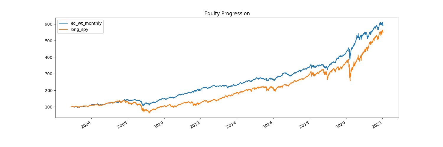
At first glance, this portfolio seems like it does a lot better! And, fortunately, we have a lot more data here - all the way since 2004. However, looking at the performance statistics, we actually barely beat SPY, only by 0.5% a year. Just like our first strategy, the main difference here is our drawdowns are significantly reduced.
We could also compare this not just to the benchmark, but to our first strategy as well. We just need to add it to bt.run like so:
res = bt.run(backtest_2, backtest_1, benchmark_test)
Stat                 eq_wt_monthly    spy_virt_7030    long_spy
-------------------  ---------------  ---------------  ----------
Start                2015-04-15       2015-04-15       2015-04-15
End                  2022-01-14       2022-01-14       2022-01-14
Risk-free rate       0.00%            0.00%            0.00%

Total Return         114.77%          152.36%          150.45%
Daily Sharpe         1.20             0.89             0.85
Daily Sortino        1.88             1.45             1.28
CAGR                 11.99%           14.70%           14.57%
Max Drawdown         -16.13%          -21.75%          -33.72%
Calmar Ratio         0.74             0.68             0.43

MTD                  -2.82%           -1.23%           -2.16%
3m                   2.12%            8.87%            5.39%
6m                   2.35%            9.61%            7.25%
YTD                  -2.82%           -1.23%           -2.16%
1Y                   9.59%            25.10%           24.43%
3Y (ann.)            20.09%           21.07%           23.83%
5Y (ann.)            14.85%           19.85%           17.58%
10Y (ann.)           -                -                -
Since Incep. (ann.)  11.99%           14.70%           14.57%

Daily Sharpe         1.20             0.89             0.85
Daily Sortino        1.88             1.45             1.28
Daily Mean (ann.)    11.81%           15.16%           15.19%
Daily Vol (ann.)     9.86%            17.05%           17.81%
Daily Skew           -0.60            -0.23            -0.73
Daily Kurt           9.00             10.24            17.32
Best Day             4.32%            7.03%            9.06%
Worst Day            -5.27%           -8.56%           -10.94%

Monthly Sharpe       1.30             1.06             1.02
Monthly Sortino      3.15             2.52             1.82
Monthly Mean (ann.)  12.03%           15.01%           14.86%
Monthly Vol (ann.)   9.22%            14.18%           14.53%
Monthly Skew         0.34             0.45             -0.42
Monthly Kurt         0.31             0.27             1.47
Best Month           9.55%            12.98%           12.70%
Worst Month          -4.12%           -5.94%           -12.49%

Yearly Sharpe        1.01             1.07             1.07
Yearly Sortino       11.50            31.58            8.44
Yearly Mean          12.69%           14.68%           15.04%
Yearly Vol           12.58%           13.77%           14.11%
Yearly Skew          0.04             0.24             -0.46
Yearly Kurt          -1.63            -1.60            -1.38
Best Year            29.00%           34.44%           31.22%
Worst Year           -2.82%           -1.23%           -4.57%

Avg. Drawdown        -1.25%           -2.44%           -1.51%
Avg. Drawdown Days   18.17            26.81            14.38
Avg. Up Month        2.56%            4.01%            3.14%
Avg. Down Month      -1.80%           -2.57%           -3.85%
Win Year %           71.43%           85.71%           71.43%
Win 12m %            98.59%           84.51%           95.77%
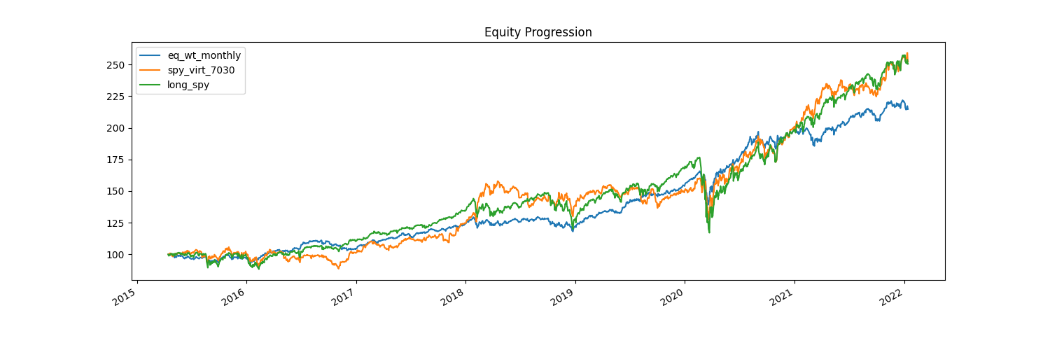
This is interesting to look at, because now we’re comparing all of the strategies, and they’ll run starting from the date of the least common denominator, which is VIRT. Now, our second strategy underperforms both of our others, but we can see that it still maintains its low volatility attributes. What might make a difference is not just the assets, but in what time period our strategy is viable.
In fact, when we do bt.algos.RunMonthly, if we look at the documentation, it states that it runs on the first trading day of each month. What if we instead offset that, and run on the last day? We could do this by adding the run_on_end_of_period=True flag to RunMonthly. How does our performance change?
name = 'eq_wt_monthly'

strategy_2 = bt.Strategy(
    name,
    [
        bt.algos.RunMonthly(run_on_end_of_period=True),
        bt.algos.SelectAll(),
        bt.algos.WeighEqually(),
        bt.algos.Rebalance()
    ]
)

eq_wt_data = data[['SPY', 'QQQ', 'TLT', 'GLD']]
eq_wt_data.dropna(inplace=True)

backtest_2 = bt.Backtest(strategy_2, eq_wt_data)
res = bt.run(backtest_2, benchmark_test)

res.plot()
res.display()
plt.show()
Stat                 eq_wt_monthly    long_spy
-------------------  ---------------  ----------
Start                2004-11-17       2004-11-17
End                  2022-01-14       2022-01-14
Risk-free rate       0.00%            0.00%

Total Return         478.20%          449.06%
Daily Sharpe         1.05             0.61
Daily Sortino        1.69             0.95
CAGR                 10.77%           10.43%
Max Drawdown         -26.86%          -55.19%
Calmar Ratio         0.40             0.19

MTD                  -2.88%           -2.16%
3m                   2.03%            5.39%
6m                   2.25%            7.25%
YTD                  -2.88%           -2.16%
1Y                   9.50%            24.43%
3Y (ann.)            19.81%           23.83%
5Y (ann.)            14.66%           17.58%
10Y (ann.)           10.90%           15.85%
Since Incep. (ann.)  10.77%           10.43%

Daily Sharpe         1.05             0.61
Daily Sortino        1.69             0.95
Daily Mean (ann.)    10.77%           11.79%
Daily Vol (ann.)     10.30%           19.22%
Daily Skew           -0.20            -0.07
Daily Kurt           7.40             16.53
Best Day             5.10%            14.52%
Worst Day            -5.37%           -10.94%

Monthly Sharpe       1.16             0.76
Monthly Sortino      2.29             1.27
Monthly Mean (ann.)  10.71%           11.06%
Monthly Vol (ann.)   9.20%            14.52%
Monthly Skew         -0.43            -0.66
Monthly Kurt         2.52             1.82
Best Month           9.04%            12.70%
Worst Month          -12.50%          -16.52%

Yearly Sharpe        1.01             0.68
Yearly Sortino       3.41             1.29
Yearly Mean          10.67%           11.14%
Yearly Vol           10.53%           16.46%
Yearly Skew          -0.47            -1.34
Yearly Kurt          0.22             3.16
Best Year            28.35%           32.31%
Worst Year           -13.16%          -36.79%

Avg. Drawdown        -1.26%           -1.70%
Avg. Drawdown Days   19.87            21.28
Avg. Up Month        2.41%            3.14%
Avg. Down Month      -1.81%           -3.59%
Win Year %           83.33%           83.33%
Win 12m %            90.82%           85.71%
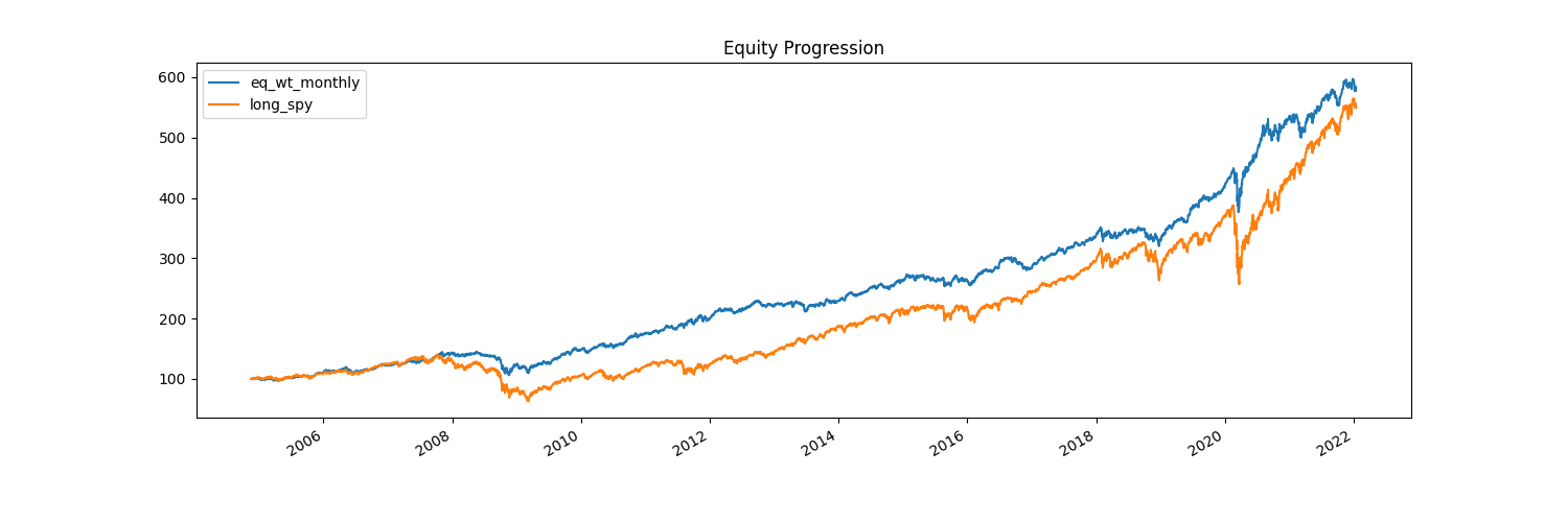 On the whole, our strategy’s performance doesn’t change that much, but we can see that our CAGR drops slightly, which reduces our overall performance by nearly 20% over the lifetime of the strategy. Even small shifts in days when we choose to execute can have an impact on our performance, and it’s important to be aware of the bias of market timing in this way.
Let’s move on to our next strategy.
Strategy 3 - Sell half when SPY goes up >2% in one day, rebuy only when SPY goes down >2% in one day
Here, we only need SPY data, but we’re going to make some changes from our previous strategies in order to provide the signal for buying and selling SPY.
In order to know what percentage SPY moves, we need to set up a separate column showing returns. In this case, we’ll use simple returns (p1/p0 - 1), since we just need to see the day-to-day changes and we’re not aggregating them, otherwise we’d use log returns. You can read more about simple versus log returns here, as well as plenty of other sources if you’re curious.
Anyways, we need to generate the returns, which we can do using pandas quite easily - we can call this column SPY_ret.
# We're going to isolate our data here first, and then drop nulls,
# since we need this series for the weights with the proper dates
spy_hl_data = data[['SPY']]
spy_hl_data.dropna(inplace=True)

# Generate returns and isolate the return series for simplicity
spy_ret = (spy_hl_data['SPY']/spy_hl_data['SPY'].shift(1)) - 1

# Rename for validation later
spy_ret.rename('SPY_returns', inplace=True)
Now, let’s create our target weights. We’ll be using bt.algos.WeightTarget to assign our weights for every specific day. This expects a dataframe, with columns of weights for each day (or lack thereof), columns being named for their asset.
# Create our weights series for SPY by copying the SPY price series
target_weights = spy_hl_data['SPY'].copy()

# Let's clear it and set all of them to None (you'll see why)
target_weights[:] = None

# We're going to start our strategy on day 1 with 100% SPY, so let's set the first weight to 1.0 (100%)
target_weights.iloc[0] = 1.0

# Now we need to fill in the dates where we know we want to make a change:
# If SPY drops 2% or more, cut or keep our allocation at half SPY, half cash
target_weights[spy_ret <= -0.02] = 0.5

# If SPY gains 2% or more, increase our allocation back to 100%
target_weights[spy_ret >= 0.02] = 1.0

# Weights need to be a DataFrame, not a series
target_weights = pd.DataFrame(target_weights)
Now, we have a dataframe, with a single column named SPY, with weights assigned to each day that fit the criteria. But what about the days where SPY is between -2% and 2%? Those are still set to None.
If we want to check this, we can just combine the prices, the returns, and the weights and see what it looks like.
# Let's make sure our prices, returns, and weights look ok
validation = pd.concat([spy_hl_data, spy_ret, target_weights], axis=1)
print(validation.tail(50))
                   SPY  SPY_returns  SPY
Date
2021-11-04  465.275391     0.004713  NaN
2021-11-05  466.889709     0.003470  NaN
2021-11-08  467.288300     0.000854  NaN
2021-11-09  465.743744    -0.003305  NaN
2021-11-10  461.996887    -0.008045  NaN
2021-11-11  462.146362     0.000324  NaN
2021-11-12  465.634094     0.007547  NaN
2021-11-15  465.793549     0.000342  NaN
2021-11-16  467.637085     0.003958  NaN
2021-11-17  466.501099    -0.002429  NaN
2021-11-18  468.085510     0.003396  NaN
2021-11-19  467.248474    -0.001788  NaN
2021-11-22  465.933075    -0.002815  NaN
2021-11-23  466.550903     0.001326  NaN
2021-11-24  467.796509     0.002670  NaN
2021-11-26  457.363190    -0.022303  0.5
2021-11-29  462.973480     0.012267  NaN
2021-11-30  453.965118    -0.019458  NaN
2021-12-01  448.922821    -0.011107  NaN
2021-12-02  455.798676     0.015316  NaN
2021-12-03  451.832611    -0.008701  NaN
2021-12-06  457.183807     0.011843  NaN
2021-12-07  466.640594     0.020685  1.0
2021-12-08  467.876221     0.002648  NaN
2021-12-09  464.717346    -0.006752  NaN
2021-12-10  469.091949     0.009413  NaN
2021-12-13  464.936584    -0.008858  NaN
2021-12-14  461.737793    -0.006880  NaN
2021-12-15  468.952454     0.015625  NaN
2021-12-16  464.816986    -0.008819  NaN
2021-12-17  459.869995    -0.010643  NaN
2021-12-20  454.980011    -0.010633  NaN
2021-12-21  463.059998     0.017759  NaN
2021-12-22  467.690002     0.009999  NaN
2021-12-23  470.600006     0.006222  NaN
2021-12-27  477.260010     0.014152  NaN
2021-12-28  476.869995    -0.000817  NaN
2021-12-29  477.480011     0.001279  NaN
2021-12-30  476.160004    -0.002765  NaN
2021-12-31  474.959991    -0.002520  NaN
2022-01-03  477.709991     0.005790  NaN
2022-01-04  477.549988    -0.000335  NaN
2022-01-05  468.380005    -0.019202  NaN
2022-01-06  467.940002    -0.000939  NaN
2022-01-07  466.089996    -0.003954  NaN
2022-01-10  465.510010    -0.001244  NaN
2022-01-11  469.750000     0.009108  NaN
2022-01-12  471.019989     0.002704  NaN
2022-01-13  464.529999    -0.013779  NaN
2022-01-14  464.720001     0.000409  NaN
We can see that we have prices, their returns, and weights, but most of the weights are empty, as promised. Is this a problem? Yes.
To fix this, we can fill our weights forward. This means that we could fill in our nulls by going down the list of dates and assigning each empty weight the last known non-null value.
target_weights.ffill(inplace=True)
We can double check again
print(target_weights.tail(10))
            SPY
Date
2022-01-03  1.0
2022-01-04  1.0
2022-01-05  1.0
2022-01-06  1.0
2022-01-07  1.0
2022-01-10  1.0
2022-01-11  1.0
2022-01-12  1.0
2022-01-13  1.0
2022-01-14  1.0
and we see that every day has a weight.
Now, we can continue as usual by setting up the bt strategy, and this should be easily recognizable by now. The only changes here are we’re using bt.algos.WeighTarget instead of bt.algos.WeighEqually as we did before, and we’re passing in the target_weights we built.
name = 'spy_high_low'

strategy_3 = bt.Strategy(
    name,
    [
        bt.algos.RunDaily(),
        bt.algos.SelectAll(),
        bt.algos.WeighTarget(target_weights),
        bt.algos.Rebalance()
    ]
)

backtest_3 = bt.Backtest(strategy_3, spy_hl_data)
res = bt.run(backtest_3, benchmark_test)

res.plot()
res.plot_weights() # Let's also plot our weights this time
res.display()
plt.show()
Stat                 spy_high_low    long_spy
-------------------  --------------  ----------
Start                1993-01-28      1993-01-28
End                  2022-01-14      2022-01-14
Risk-free rate       0.00%           0.00%

Total Return         602.16%         1713.34%
Daily Sharpe         0.54            0.63
Daily Sortino        0.83            0.99
CAGR                 6.96%           10.52%
Max Drawdown         -44.30%         -55.19%
Calmar Ratio         0.16            0.19

MTD                  -2.16%          -2.16%
3m                   2.48%           5.39%
6m                   3.43%           7.25%
YTD                  -2.16%          -2.16%
1Y                   13.28%          24.43%
3Y (ann.)            12.02%          23.83%
5Y (ann.)            10.07%          17.58%
10Y (ann.)           10.19%          15.85%
Since Incep. (ann.)  6.96%           10.52%

Daily Sharpe         0.54            0.63
Daily Sortino        0.83            0.99
Daily Mean (ann.)    7.79%           11.76%
Daily Vol (ann.)     14.53%          18.71%
Daily Skew           -0.54           -0.06
Daily Kurt           11.87           12.15
Best Day             7.26%           14.52%
Worst Day            -10.94%         -10.94%

Monthly Sharpe       0.63            0.76
Monthly Sortino      1.04            1.29
Monthly Mean (ann.)  7.44%           11.10%
Monthly Vol (ann.)   11.83%          14.57%
Monthly Skew         -0.65           -0.62
Monthly Kurt         2.83            1.27
Best Month           11.33%          12.70%
Worst Month          -17.17%         -16.52%

Yearly Sharpe        0.59            0.66
Yearly Sortino       1.30            1.45
Yearly Mean          7.56%           11.72%
Yearly Vol           12.74%          17.70%
Yearly Skew          -0.72           -0.83
Yearly Kurt          0.40            0.61
Best Year            26.94%          38.05%
Worst Year           -26.85%         -36.79%

Avg. Drawdown        -1.73%          -1.87%
Avg. Drawdown Days   34.67           25.57
Avg. Up Month        2.55%           3.28%
Avg. Down Month      -2.70%          -3.54%
Win Year %           68.97%          79.31%
Win 12m %            77.22%          82.25%
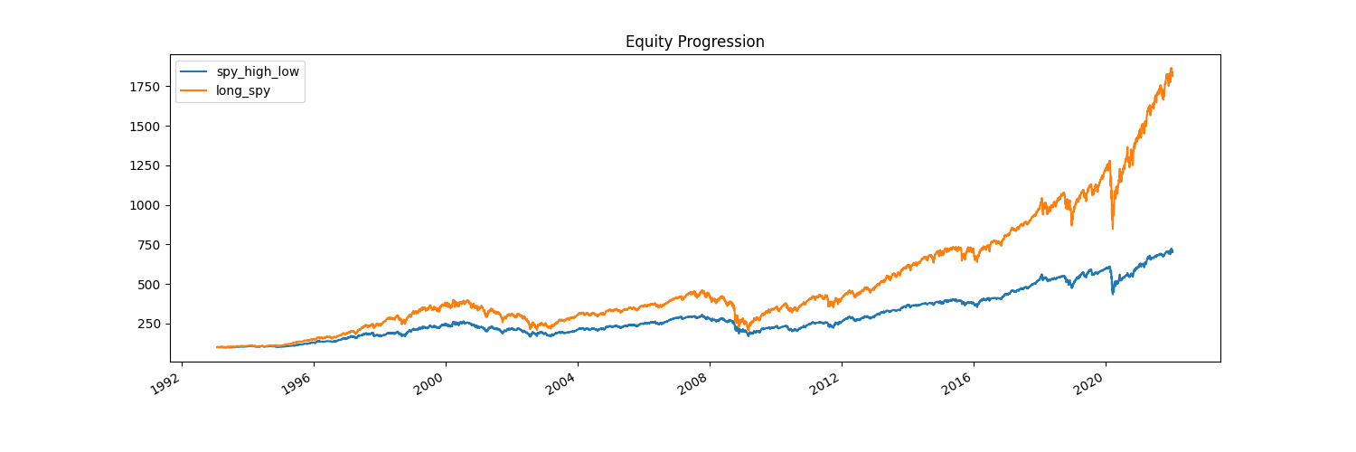
Let’s look at the results. This is pretty disastrous! Buying when it goes up and selling when it goes down by 2% is clearly a poor strategy. We reduce our volatility relative to the benchmark, but not as much as our previous ones, and at the cost of a significantly reduced return. We drawdown for longer periods of time, and our maximum drawdown is nearly the same as holding SPY.
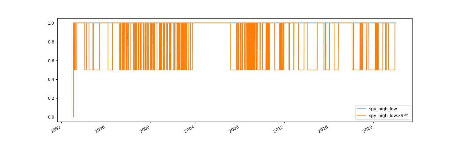
What can we do better? Let’s first see how often we’re actually at half allocation. I opted to add in plotting the weights this time, so we can see how our allocation changed. We jump around from 50% to 100%, and we can see that we actually spend quite a bit of time at 50%.
# How many days are our target weights at 0.5 divided by the total number of days
print(target_weights[target_weights == 0.5].count()/len(target_weights))
SPY 0.406443
We’re half allocated nearly 40% of the time! Could we maybe reduce the percentages to 1% to see if that could improve performance? To do that, we just need to change the parameter in target_weights to 0.01 instead of 0.02, and rerun our test.
target_weights[spy_ret <= -0.01] = 0.5
target_weights[spy_ret >= 0.01] = 1.0
Stat                 spy_high_low    long_spy
-------------------  --------------  ----------
Start                1993-01-28      1993-01-28
End                  2022-01-14      2022-01-14
Risk-free rate       0.00%           0.00%

Total Return         435.63%         1713.34%
Daily Sharpe         0.47            0.63
Daily Sortino        0.72            0.99
CAGR                 5.97%           10.52%
Max Drawdown         -54.32%         -55.19%
Calmar Ratio         0.11            0.19

MTD                  -1.77%          -2.16%
3m                   4.60%           5.39%
6m                   4.46%           7.25%
YTD                  -1.77%          -2.16%
1Y                   17.05%          24.43%
3Y (ann.)            15.86%          23.83%
5Y (ann.)            12.81%          17.58%
10Y (ann.)           10.87%          15.85%
Since Incep. (ann.)  5.97%           10.52%

Daily Sharpe         0.47            0.63
Daily Sortino        0.72            0.99
Daily Mean (ann.)    6.85%           11.76%
Daily Vol (ann.)     14.47%          18.71%
Daily Skew           -0.61           -0.06
Daily Kurt           10.48           12.15
Best Day             7.26%           14.52%
Worst Day            -10.94%         -10.94%

Monthly Sharpe       0.54            0.76
Monthly Sortino      0.90            1.29
Monthly Mean (ann.)  6.55%           11.10%
Monthly Vol (ann.)   12.15%          14.57%
Monthly Skew         -0.66           -0.62
Monthly Kurt         2.12            1.27
Best Month           9.25%           12.70%
Worst Month          -17.17%         -16.52%

Yearly Sharpe        0.47            0.66
Yearly Sortino       0.84            1.45
Yearly Mean          6.90%           11.72%
Yearly Vol           14.77%          17.70%
Yearly Skew          -1.11           -0.83
Yearly Kurt          1.76            0.61
Best Year            27.09%          38.05%
Worst Year           -38.15%         -36.79%

Avg. Drawdown        -1.80%          -1.87%
Avg. Drawdown Days   45.22           25.56
Avg. Up Month        2.67%           3.28%
Avg. Down Month      -2.89%          -3.54%
Win Year %           68.97%          79.31%
Win 12m %            76.33%          82.25%
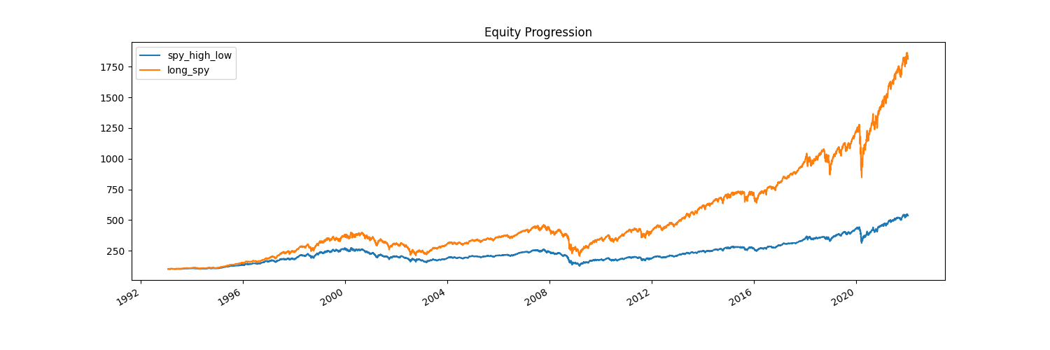 We can see that we actually performed worse than before! What if we sell only when we’re down 2% or more, and maintain 100% when we’re up 1% or more?
target_weights[spy_ret <= -0.02] = 0.5
target_weights[spy_ret >= 0.01] = 1.0
Stat                 spy_high_low    long_spy
-------------------  --------------  ----------
Start                1993-01-28      1993-01-28
End                  2022-01-14      2022-01-14
Risk-free rate       0.00%           0.00%

Total Return         887.09%         1713.34%
Daily Sharpe         0.57            0.63
Daily Sortino        0.88            0.99
CAGR                 8.23%           10.52%
Max Drawdown         -55.32%         -55.19%
Calmar Ratio         0.15            0.19

MTD                  -2.16%          -2.16%
3m                   4.75%           5.39%
6m                   6.54%           7.25%
YTD                  -2.16%          -2.16%
1Y                   21.45%          24.43%
3Y (ann.)            18.66%          23.83%
5Y (ann.)            14.81%          17.58%
10Y (ann.)           13.65%          15.85%
Since Incep. (ann.)  8.23%           10.52%

Daily Sharpe         0.57            0.63
Daily Sortino        0.88            0.99
Daily Mean (ann.)    9.24%           11.76%
Daily Vol (ann.)     16.28%          18.71%
Daily Skew           -0.57           -0.06
Daily Kurt           8.27            12.15
Best Day             7.26%           14.52%
Worst Day            -10.94%         -10.94%

Monthly Sharpe       0.65            0.76
Monthly Sortino      1.07            1.29
Monthly Mean (ann.)  8.87%           11.10%
Monthly Vol (ann.)   13.69%          14.57%
Monthly Skew         -0.73           -0.62
Monthly Kurt         1.90            1.27
Best Month           11.33%          12.70%
Worst Month          -17.17%         -16.52%

Yearly Sharpe        0.55            0.66
Yearly Sortino       1.07            1.45
Yearly Mean          9.47%           11.72%
Yearly Vol           17.18%          17.70%
Yearly Skew          -0.97           -0.83
Yearly Kurt          1.30            0.61
Best Year            38.05%          38.05%
Worst Year           -40.98%         -36.79%

Avg. Drawdown        -1.89%          -1.87%
Avg. Drawdown Days   31.85           25.57
Avg. Up Month        3.06%           3.28%
Avg. Down Month      -3.30%          -3.54%
Win Year %           72.41%          79.31%
Win 12m %            79.88%          82.25%
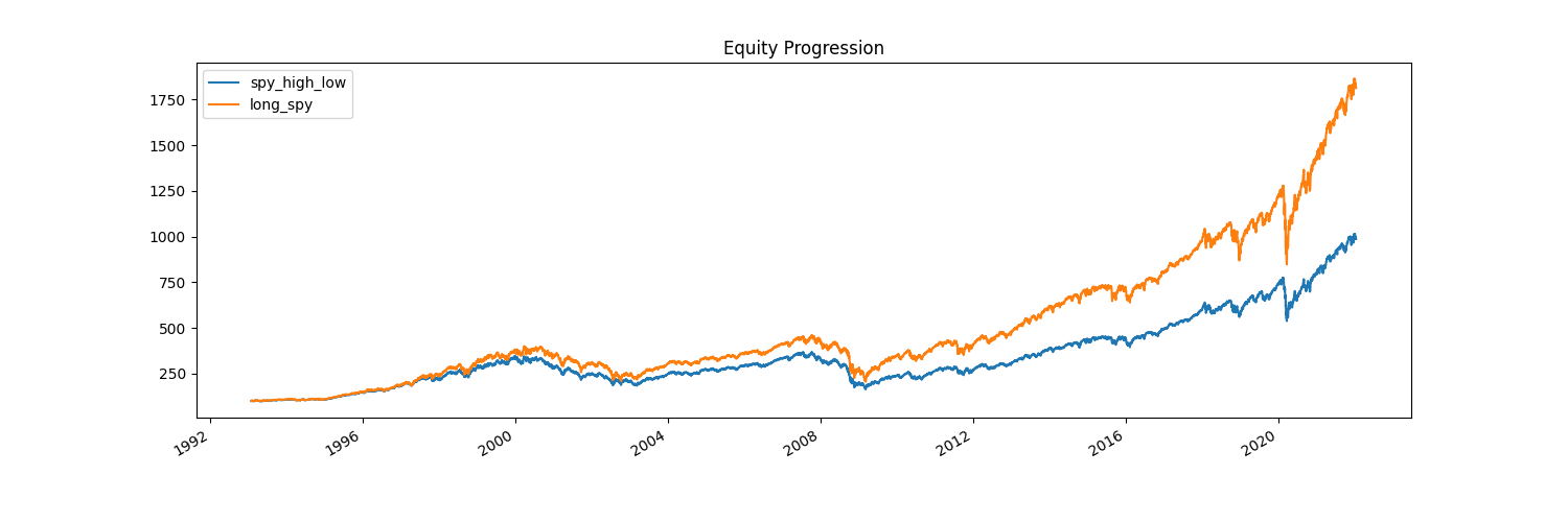 Now our volatility and drawdowns are actually worse, and we’re still not beating our benchmark.
What if we switch around the strategy? Buy when SPY drops, and sell when it goes up? Let’s keep the down 2%/ up 1% numbers.
target_weights[spy_ret <= -0.02] = 1.0
target_weights[spy_ret >= 0.01] = 0.5
Stat                 spy_high_low    long_spy
-------------------  --------------  ----------
Start                1993-01-28      1993-01-28
End                  2022-01-14      2022-01-14
Risk-free rate       0.00%           0.00%

Total Return         796.94%         1713.34%
Daily Sharpe         0.64            0.63
Daily Sortino        1.03            0.99
CAGR                 7.87%           10.52%
Max Drawdown         -32.32%         -55.19%
Calmar Ratio         0.24            0.19

MTD                  -1.08%          -2.16%
3m                   3.35%           5.39%
6m                   4.36%           7.25%
YTD                  -1.08%          -2.16%
1Y                   14.53%          24.43%
3Y (ann.)            16.82%          23.83%
5Y (ann.)            11.56%          17.58%
10Y (ann.)           10.08%          15.85%
Since Incep. (ann.)  7.87%           10.52%

Daily Sharpe         0.64            0.63
Daily Sortino        1.03            0.99
Daily Mean (ann.)    8.44%           11.76%
Daily Vol (ann.)     13.15%          18.71%
Daily Skew           0.95            -0.06
Daily Kurt           36.59           12.15
Best Day             14.52%          14.52%
Worst Day            -9.57%          -10.94%

Monthly Sharpe       0.85            0.76
Monthly Sortino      1.37            1.29
Monthly Mean (ann.)  8.03%           11.10%
Monthly Vol (ann.)   9.41%           14.57%
Monthly Skew         -0.83           -0.62
Monthly Kurt         3.69            1.27
Best Month           10.45%          12.70%
Worst Month          -12.14%         -16.52%

Yearly Sharpe        0.82            0.66
Yearly Sortino       2.16            1.45
Yearly Mean          8.05%           11.72%
Yearly Vol           9.87%           17.70%
Yearly Skew          -0.52           -0.83
Yearly Kurt          0.13            0.61
Best Year            26.12%          38.05%
Worst Year           -15.18%         -36.79%

Avg. Drawdown        -1.04%          -1.87%
Avg. Drawdown Days   18.33           25.50
Avg. Up Month        1.95%           3.29%
Avg. Down Month      -2.20%          -3.51%
Win Year %           82.76%          79.31%
Win 12m %            82.84%          82.25%
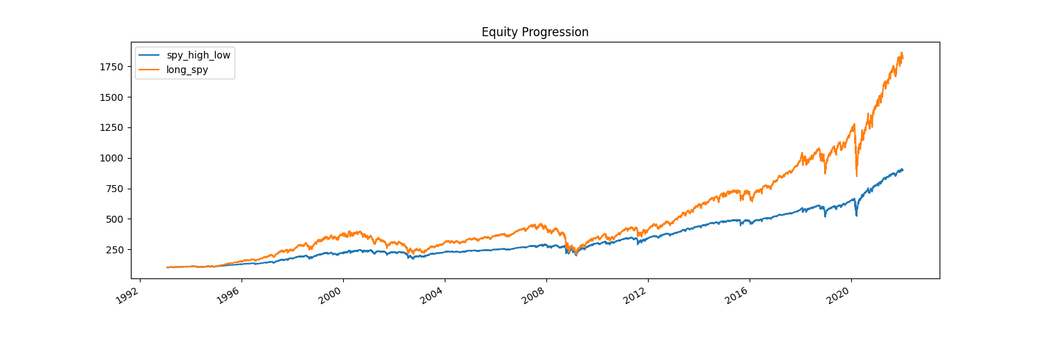 This time we perform better but we’re actually half allocated nearly 90% of the time. Let’s try one final adjustment, which is that we become half allocated only when the market jumps 2% or more, and otherwise we’re 100% allocated.
target_weights[spy_ret < 0.02] = 1.0
target_weights[spy_ret >= 0.02] = 0.5
Stat                 spy_high_low    long_spy
-------------------  --------------  ----------
Start                1993-01-28      1993-01-28
End                  2022-01-14      2022-01-14
Risk-free rate       0.00%           0.00%

Total Return         2104.61%        1713.34%
Daily Sharpe         0.68            0.63
Daily Sortino        1.08            0.99
CAGR                 11.27%          10.52%
Max Drawdown         -51.47%         -55.19%
Calmar Ratio         0.22            0.19

MTD                  -2.16%          -2.16%
3m                   5.25%           5.39%
6m                   7.10%           7.25%
YTD                  -2.16%          -2.16%
1Y                   24.75%          24.43%
3Y (ann.)            31.04%          23.83%
5Y (ann.)            21.72%          17.58%
10Y (ann.)           17.65%          15.85%
Since Incep. (ann.)  11.27%          10.52%

Daily Sharpe         0.68            0.63
Daily Sortino        1.08            0.99
Daily Mean (ann.)    12.35%          11.76%
Daily Vol (ann.)     18.22%          18.71%
Daily Skew           0.06            -0.06
Daily Kurt           12.18           12.15
Best Day             14.52%          14.52%
Worst Day            -9.84%          -10.94%

Monthly Sharpe       0.82            0.76
Monthly Sortino      1.44            1.29
Monthly Mean (ann.)  11.73%          11.10%
Monthly Vol (ann.)   14.24%          14.57%
Monthly Skew         -0.47           -0.62
Monthly Kurt         1.23            1.27
Best Month           15.40%          12.70%
Worst Month          -14.90%         -16.52%

Yearly Sharpe        0.67            0.66
Yearly Sortino       1.56            1.45
Yearly Mean          12.64%          11.72%
Yearly Vol           18.93%          17.70%
Yearly Skew          -0.63           -0.83
Yearly Kurt          0.06            0.61
Best Year            40.48%          38.05%
Worst Year           -34.94%         -36.79%

Avg. Drawdown        -1.89%          -1.87%
Avg. Drawdown Days   24.52           25.50
Avg. Up Month        3.28%           3.28%
Avg. Down Month      -3.39%          -3.54%
Win Year %           79.31%          79.31%
Win 12m %            81.36%          82.25%
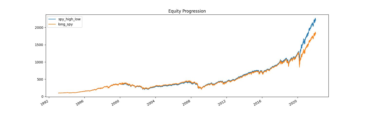 Now, we have some interesting results! We’re only half allocated ~3-4% of the time and for the most part we either slightly under or outperform the benchmark. We take on some more volatility, but we end up outperforming quite heavily, especially over the last two years.
While this could be for any number of reasons, it’s important to avoid the trap of constructing specific signals (which is what we did) based on what happened in the past. We could, if we wanted to, find ranges of percentages preceding drops, set weights there to be 0.5, 0.0, or even -1.0 (to short), and long otherwise. If we did so, we’d just be gaming our backtests to look as good as possible and it wouldn’t necessarily or even likely work going forward.
However, feel free to play around and tinker with this sort of stuff - change weights to -1.0 for a 100% short position, change the percentage ranges, etc.
Strategy 4 - UVXY Long/Short based on VIX and the VX front
Let’s move on to the last strategy here. We’re going to be trading two assets, SPY and UVXY.
From the ETF manager, UVXY does the following:
The Funds are benchmarked to an Index of VIX futures contracts.
The Funds are not benchmarked to the widely referenced Cboe Volatility Index, commonly known as the “VIX.”

This leveraged ProShares ETF seeks a return that is 1.5x the return of its underlying benchmark (target) for a single day,
as measured from one NAV calculation to the next.

ProShares Ultra VIX Short-Term Futures ETF provides leveraged exposure to the S&P 500 VIX Short-Term Futures Index,
which measures the returns of a portfolio of monthly VIX futures contracts with a weighted average of one month to expiration.
So, this is a levered short-term VIX futures ETF. VIX futures trade under VX, but we’ll need the VIX index as well.
The idea is to look at the VIX index and the closest but greater than 30-day current VIX future (VX). We’re going to be short at half by default, but if the VIX index is higher than the price of that future by more than 10%, we long UVXY at a weight of 1.0.
As I mentioned earlier, we can actually create a strategy of strategies, which we’ll do here as we also want to combine this with a long-only SPY strategy. Then, we’ll rebalance both of these daily to 50/50 between the two.
Now, to do this we need data on SPY, UVXY, and VIX, which we already have from yfinance. However, we also need data on the VIX futures, and we need the series of each of them, as, according to our strategy, we need to select the closest expiry future that’s at least 30 days out.
The provider of the VIX, CBOE, offers historical data for download on their official page here.
Manually downloading these would be quite annoying, so we can automatically fetch and load them in, and create a continuous price series of futures prices. I’m not going to go over this directly in this post, so I’m just going to attach the stitched together series as a .csv for your purposes. You can get it from my repo here.
But specifically, I went through the files, sorted by expiry, and took the closing price for each of those expiries so long as they were before 30 days to the expiry itself. Then, I moved on to the next available expiry and repeated the process to get one continuous series.
Now, to use this data, we just load it in like the others, except this time we’re using the pandas read_csv method:
# Load in our VX continuous futures stream from our CSV,
# specifying the 'Date' column as the index and converting it to datetime (so we can concat)
vx_cont = pd.read_csv('vx_cont.csv', index_col='Date')
vx_cont.index = pd.to_datetime(vx_cont.index)

# Add the VX cont series to our data
data = pd.concat([data, vx_cont], axis=1)
Now, we can isolate our data for strategy 4 and define it.
# Isolate the UVXY, VIX, and VX_CONT into their own dataset
strategy_4_data = data[['UVXY', '^VIX', 'VX_CONT']]

# Drop nulls so that we only have common data remaining
strategy_4_data.dropna(inplace=True)

# Split out the VIX and VX_CONT for simplicity
vix_spot = strategy_4_data['^VIX']
vix_fut = strategy_4_data['VX_CONT']

# Define the target weights
tw = vix_fut.copy()

# We want to be short by default at half
tw[:] = -0.5

# When current VIX greater than the closest future by more than 10%, revert and go fully long
tw[vix_spot/vix_fut > 1.1] = 1.0

# Convert our weights to a dataframe
tw = pd.DataFrame(tw)

# Rename the column so that it matches the instrument we're using (UVXY)
tw.columns = ['UVXY']

# Define the UVXY strategy
name = 'uvxy_dynamic'
strategy_4_uvxy = bt.Strategy(
    name,
    [
        bt.algos.WeighTarget(tw),
        bt.algos.Rebalance()
    ]
)

# Set up the backtest
uvxy_dynamic = bt.Backtest(strategy_4_uvxy, strategy_4_data[['UVXY']], integer_positions=False)
Most of this should make sense, except notice here I indicated that integer_positions=False. This is because strategies are allocated $1M by default in backtests, and since UVXY has gone through so many reverse splits, the initial historical data for it puts it at a ridiculously high price. You can verify this for yourself:
print(strategy_4_data['UVXY'].head(10))
Date
2013-01-02    16070000.0
2013-01-03    15930000.0
2013-01-04    15300000.0
2013-01-07    15270000.0
2013-01-08    14960000.0
2013-01-09    14980000.0
2013-01-10    14270000.0
2013-01-11    14160000.0
2013-01-14    13730000.0
2013-01-15    13670000.0
Name: UVXY, dtype: float64
As a result, we wouldn’t be able to long or short even one share fully, thus we need to tell bt that we’re okay with fractional allocations.
Let’s run this strategy against our benchmark.
res = bt.run(uvxy_dynamic, benchmark_test)
res.display()
res.plot()
res.plot_weights()
plt.show()
Stat                 uvxy_dynamic    long_spy
-------------------  --------------  ----------
Start                2013-01-02      2013-01-02
End                  2022-01-13      2022-01-13
Risk-free rate       0.00%           0.00%

Total Return         2314.35%        276.82%
Daily Sharpe         0.82            0.98
Daily Sortino        1.40            1.48
CAGR                 42.28%          15.83%
Max Drawdown         -82.47%         -33.72%
Calmar Ratio         0.51            0.47

MTD                  -1.60%          -2.20%
3m                   -6.12%          7.12%
6m                   1.88%           7.36%
YTD                  -1.60%          -2.20%
1Y                   48.30%          23.94%
3Y (ann.)            70.45%          23.83%
5Y (ann.)            55.38%          17.46%
10Y (ann.)           42.28%          15.83%
Since Incep. (ann.)  42.28%          15.83%

Daily Sharpe         0.82            0.98
Daily Sortino        1.40            1.48
Daily Mean (ann.)    65.62%          16.05%
Daily Vol (ann.)     79.64%          16.42%
Daily Skew           2.22            -0.73
Daily Kurt           32.54           18.27
Best Day             66.21%          9.06%
Worst Day            -33.45%         -10.94%

Monthly Sharpe       0.75            1.16
Monthly Sortino      1.78            2.10
Monthly Mean (ann.)  61.18%          15.43%
Monthly Vol (ann.)   81.34%          13.32%
Monthly Skew         2.63            -0.45
Monthly Kurt         16.59           1.80
Best Month           155.50%         12.70%
Worst Month          -50.24%         -12.49%

Yearly Sharpe        0.62            1.02
Yearly Sortino       5.72            8.30
Yearly Mean          45.24%          13.32%
Yearly Vol           73.54%          13.05%
Yearly Skew          1.25            -0.08
Yearly Kurt          0.77            -1.37
Best Year            193.26%         31.22%
Worst Year           -18.12%         -4.57%

Avg. Drawdown        -14.05%         -1.45%
Avg. Drawdown Days   73.16           13.13
Avg. Up Month        15.66%          3.06%
Avg. Down Month      -13.60%         -3.34%
Win Year %           55.56%          77.78%
Win 12m %            70.41%          93.88%
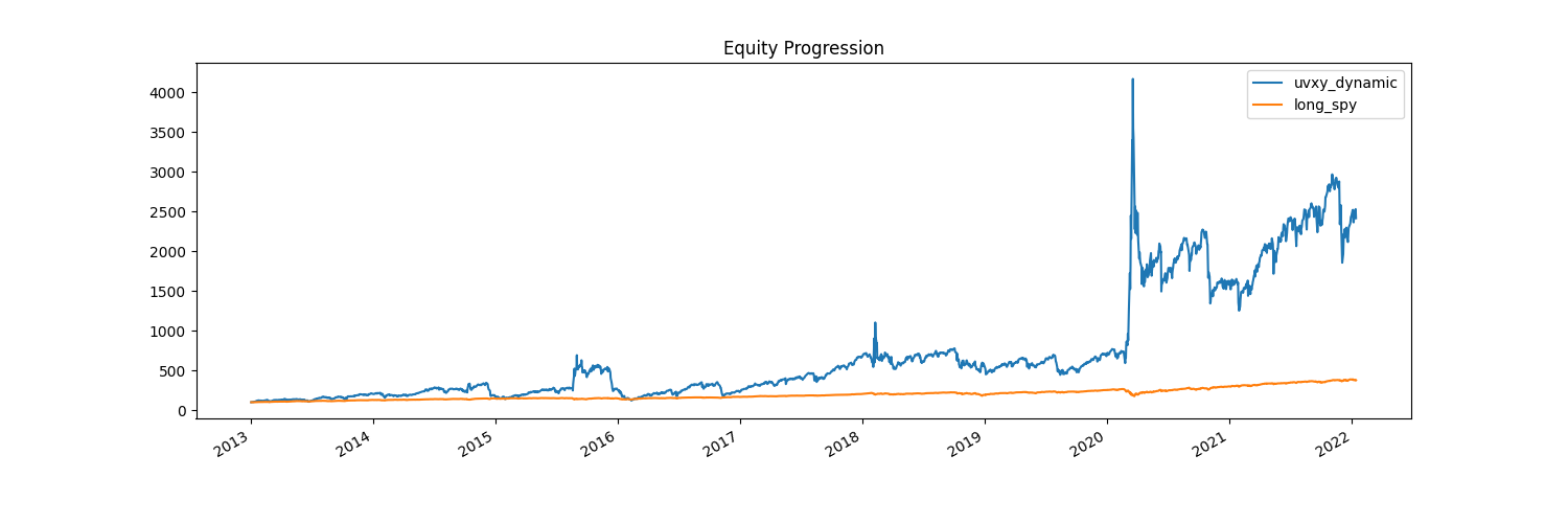
Wow! This seems to perform very well, at the cost of incredibly large drawdowns (-82%) and incredibly high volatility. This is not something many would be comfortable with.
Let’s see if combining this strategy with a pure long SPY would help us reduce some of the volatility and capture some of the excess returns.
To do this, we can combine the output our previous bt.run and extract the price data to create synthetic securities, then rebalance their weights like we would any with any other instrument.
So,
# Once we ran the previous backtest, we can extract the prices data to create synthetic securities
synthetic = bt.merge(res['uvxy_dynamic'].prices, res['long_spy'].prices)

# This is our new data, which is essentially the equity curve of each sub-strategy we tested.
# We can use this data to test our final strategy, just as before.
strategy_4 = bt.Strategy(
    'combined_uvxy_spy',
    [
        bt.algos.SelectAll(),
        bt.algos.WeighSpecified(uvxy_dynamic=0.5, long_spy=0.5),
        bt.algos.Rebalance()
    ]
)

# Create and run
t = bt.Backtest(strategy_4, synthetic, integer_positions=False)
res = bt.run(t, benchmark_test)

# Display summary statistics and plot the weights
res.display()
res.plot()
res.plot_weights()
plt.show()
Stat                 combined_uvxy_spy    long_spy
-------------------  -------------------  ----------
Start                2013-01-02           2013-01-02
End                  2022-01-13           2022-01-13
Risk-free rate       0.00%                0.00%

Total Return         1786.61%             276.82%
Daily Sharpe         1.00                 0.98
Daily Sortino        1.62                 1.48
CAGR                 38.45%               15.83%
Max Drawdown         -56.72%              -33.72%
Calmar Ratio         0.68                 0.47

MTD                  -1.85%               -2.20%
3m                   1.42%                7.12%
6m                   6.34%                7.36%
YTD                  -1.85%               -2.20%
1Y                   39.76%               23.94%
3Y (ann.)            58.56%               23.83%
5Y (ann.)            47.60%               17.46%
10Y (ann.)           38.45%               15.83%
Since Incep. (ann.)  38.45%               15.83%

Daily Sharpe         1.00                 0.98
Daily Sortino        1.62                 1.48
Daily Mean (ann.)    40.84%               16.05%
Daily Vol (ann.)     40.95%               16.42%
Daily Skew           0.99                 -0.73
Daily Kurt           19.28                18.27
Best Day             31.01%               9.06%
Worst Day            -15.74%              -10.94%

Monthly Sharpe       0.96                 1.16
Monthly Sortino      2.07                 2.10
Monthly Mean (ann.)  39.92%               15.43%
Monthly Vol (ann.)   41.53%               13.32%
Monthly Skew         1.70                 -0.45
Monthly Kurt         11.68                1.80
Best Month           74.22%               12.70%
Worst Month          -29.16%              -12.49%

Yearly Sharpe        0.89                 1.02
Yearly Sortino       58.00                8.30
Yearly Mean          35.67%               13.32%
Yearly Vol           40.07%               13.05%
Yearly Skew          0.94                 -0.08
Yearly Kurt          -0.41                -1.37
Best Year            105.34%              31.22%
Worst Year           -1.85%               -4.57%

Avg. Drawdown        -5.71%               -1.44%
Avg. Drawdown Days   35.32                13.07
Avg. Up Month        8.91%                3.06%
Avg. Down Month      -7.39%               -3.34%
Win Year %           88.89%               77.78%
Win 12m %            87.76%               93.88%
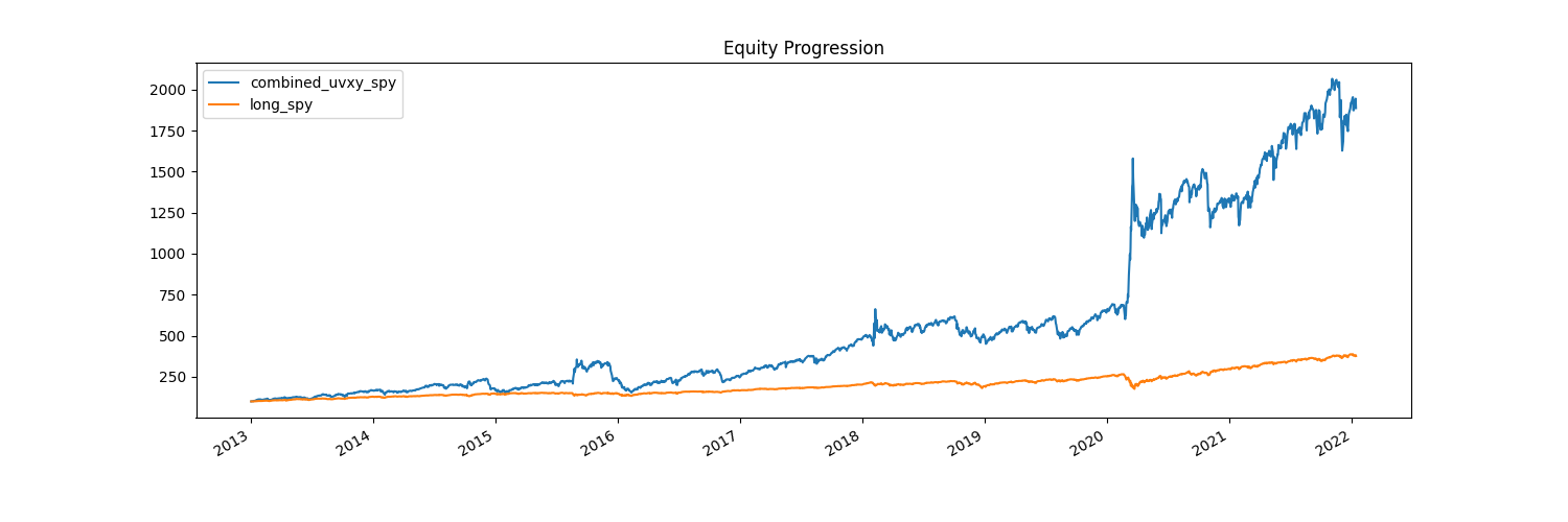 The performance is better! We keep most of the excess returns from the dynamic UVXY strategy and reduce our drawdown. However, this is still something most people wouldn’t be comfortable with investing in, with a max drawdown of ~57%.
Feel free to tinker with the weights of each of the strategies (maybe 70/30 is better?) or the UVXY long/short logic, but hopefully this gives you an idea of how to combine multiple strategies into one, as well as working with external data.
Conclusion
While backtesting isn’t perfect, it’s still an important part of research before deploying a new strategy. Performing backtests helps us see how our strategies would’ve likely worked in the past, and provide direct insight on the actual, measured performance. However, we need to be careful about how we’re constructing our strategies, keeping biases in mind, as well as considering the quality of our data.
With the examples and information here, you should now be fairly comfortable with pulling historical data and using it to test whatever strategy you can think of using bt. I recommend reading further into the documentation for bt here, as there are many algos and additional bt features I didn’t cover. In a later post, I’ll go over fetching data from the Interactive Brokers API, which you could use in your backtests as well.
The full code is also available on my github here.
Obligatory disclaimer, none of this is investment advice.
References
yfinanceDocumentationbtDocumentation- UVXY Description
- CBOE Historical VX Data